(Updated October 2023)
G100
version 7.1
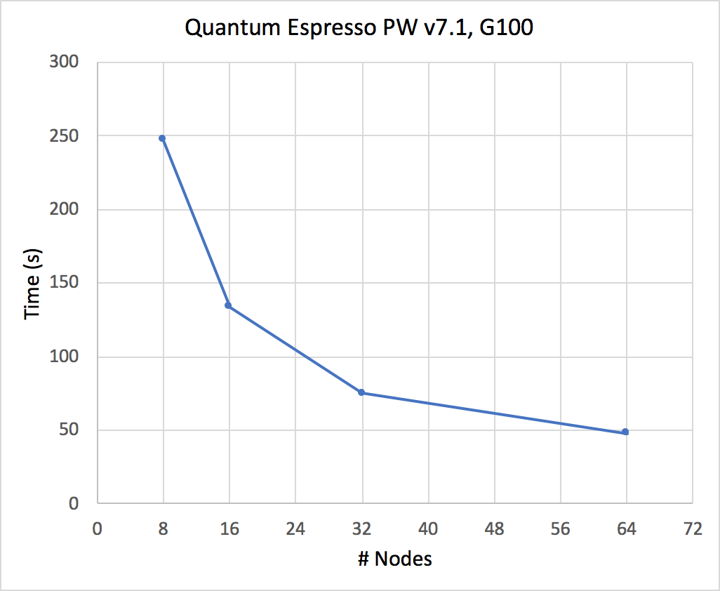
CNT10POR8 : R&G scaling on the CPU
- Performance analysis for a a Carbon nanotube functionalized with two porphyrine molecules, about 1500 atoms, 8000 bands, 1 k-point
- The average time per iteration is reported as a function of the number of nodes.
N° nodes | Time (s) |
| 8 | 248 |
| 16 | 134 |
| 32 | 75 |
| 64 | 48 |
Graphic 1: the QE performance (simulation time in s) is reported vs. the increasing number of nodes
Leonardo
version 7.2
CNT10POR8 : R&G scaling on the GPUs
- Performance analysis for a a Carbon nanotube functionalized with two porphyrine molecules, about 1500 atoms, 8000 bands, 1 k-point.
- The average time per iteration is reported as a function of the number of nodes.
Table2: The performance of the MPI (1 task per GPU) + GPU (4 per node) + OpenMP (8 threads per task)
N° nodes | Time (s) |
| 8 | 21.34 |
| 16 | 14.06 |
| 20 | 12.18 |
| 24 | 11.60 |
Graphic 2: the QE(v7.2) performance (simulation time in s) is reported vs. the increasing number of nodes
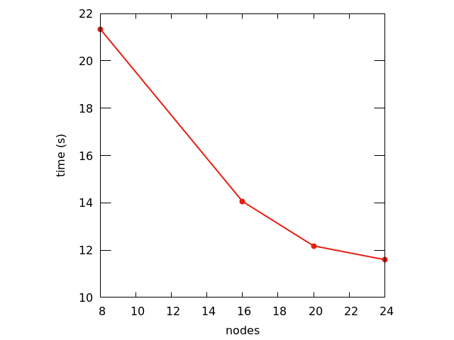
GPUs strongly improve the time to solution, but scaling with R&G has little efficiency beyond the minimum number of GPUs to be used for memory constraints.
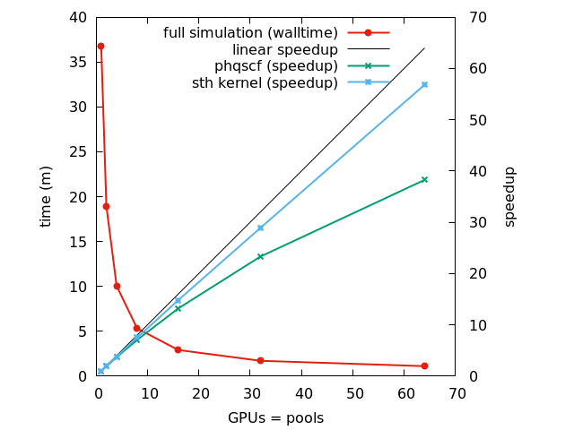
Si-16layers - all irrep : Images and pool scaling
In PHONON, TDDFPT and NEB images can be used to distribute independent calculations. In this benchmark we simulate the calculation of the dynamical matrix at a given q point for a structure of 16 layers of Silicon. The simulation computes all the contributes to the dynamical matrix from the 192 irreducible representations. By using images, we can distribute these 192 irreducible representations among MPI ranks. The perturbed system has 128 k-points, corresponding to 64 pools maximum ( kunit = 2 in this PHONON simulation ).
Thus, we can distribute the simulation up to 192 x 64 gpus = 12288 gpus = 3072 nodes.
In the following benchmark we present the time to solution (s) when distributing from 1 to 1024 nodes (colums), the efficiency of the entire simulation (black dashed line) and the efficiency of the main kernel (violet line).
| Nodes | phqscf (s) | dynmat0 (s) | solve_linter (s) | sth_kernel (s) | h_psi (s) | walltime (s) |
| 4 | 31770,01 | 36,58 | 30.897,59 | 27444,56 | 12649,38 | 31860,00 |
| 8 | 17837,22 | 34,7 | 16.981,20 | 14023,52 | 6422,33 | 17880,00 |
| 16 | 10570,72 | 31,56 | 9.766,42 | 7051,89 | 3189,66 | 10620,00 |
| 32 | 5290,35 | 30,7 | 4.891,41 | 3535,66 | 1598,94 | 5340,00 |
| 64 | 2700,97 | 31,71 | 2.496,78 | 1805,39 | 817,76 | 2733,14 |
| 128 | 1375,29 | 32,25 | 1270,39 | 917,08 | 415,09 | 1401,46 |
| 256 | 711,83 | 31,81 | 657,49 | 474,75 | 214,19 | 757,98 |
| 512 | 382,94 | 31,96 | 353,18 | 253,74 | 125,36 | 447,93 |
| 1024 | 223,69 | 31,55 | 206,78 | 148,51 | 98,76 | 319,31 |
Graphic 3: Time to solution (m) and efficiencies from 1 to 1024 nodes. The simulation is scaled on pools up to 16 nodes, then images are used to further distribute computation. The labels on top of the columns (ni,nk,npw,omp) define the parallelization used. ni : is the number of images, nk : number of pools, npw : number of R&G processes, omp : number of openmp threads.
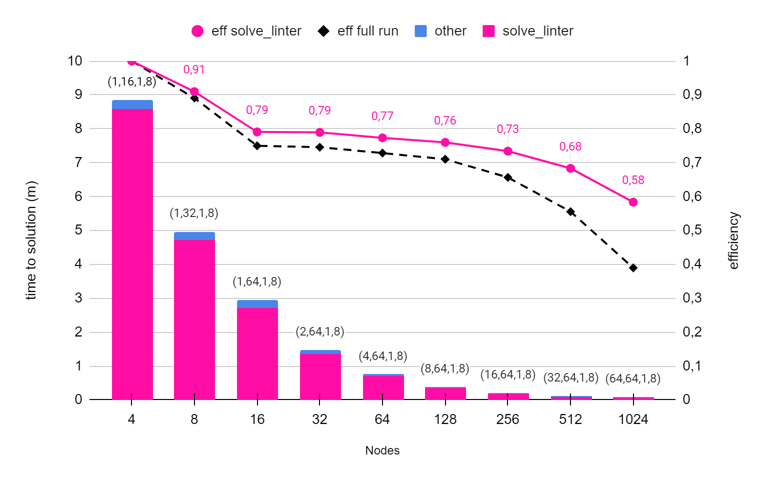
Images entail little communications, and the efficiency is well sustained up to 1024 nodes for the main kernel (solve_linter) without initialization.
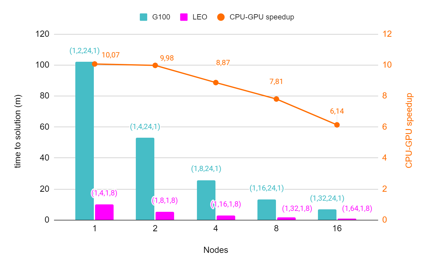
CPU (G100) vs GPU (Leonardo)
Si-16layers - 1 irrep : Pool scaling
Performance analysis of the linear response calculation in ph.x for the system benchmarked here https://gitlab.hpc.cineca.it/cineca-benchmarking/applications/-/blob/main/quantum_espresso/Leonardo/small/SI16L-workflow-irr1/plot.png.
- CPU (G100) - GPU (Leonardo) speedup
- Scaling with increasing pools ( one pool per gpu ) for a single irreducible representation
| Nodes | phqscf | ortho | sth_kernel | GPU time (s) | CPU time ref (s) |
| 1 | 2136,07 | 121,23 | 2047,89 | 2203,88 | - |
| 1 | 1099,34 | 64,39 | 1047,00 | 1137,37 | - |
| 1 | 584,01 | 34,88 | 543,51 | 607,72 | 6120,00 |
| 2 | 302,31 | 18,34 | 272,62 | 318,61 | 3179,40 |
| 4 | 161,82 | 9,68 | 138,19 | 174,65 | 1549,20 |
| 8 | 91,60 | 4,94 | 70,84 | 102,5 | 800,40 |
| 16 | 55,81 | 2,66 | 36,04 | 66,44 | 408,00 |
Graphic 4: Time to solution (m) for the CPU (G100) and GPU (Leonardo) runs from 1 to 16 nodes. CPU and GPU runs use a different parallelization, defined by the labels on top of the columns (ni,nk,npw,omp). ni : is the number of images, nk : number of pools, npw : number of R&G processes, omp : number of openmp threads. The yellow line shows the CPU-GPU speedup
Graphic 5: the QE performance (simulation time in s) is reported vs. the increasing number of nodes with different speedups
Pools scale efficiently on GPUs (this is true also for pw.x)
© Copyright 2